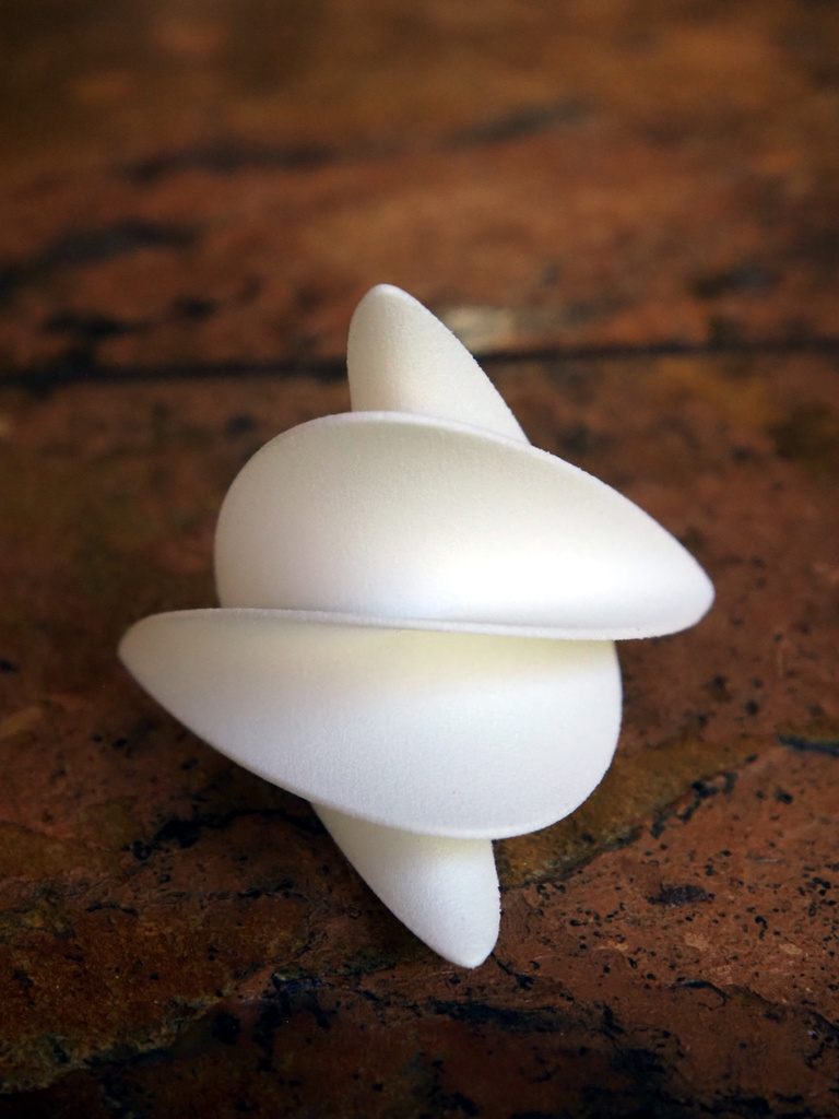
This post explains the simple complex math underlying the shape below. Is that a contradiction in terms? Not necessarily: complex refers to complex numbers, which are perhaps subtle, but not malicious.
We’ll start by reviewing rectangular coordinates and geometric interpretations, and circular functions, which you have seen if you studied trigonometry.
Circles and Coordinates
The trigonometric functions cosine and sine are shadows of circular motion. This breezy assertion has a particularly concrete geometric interpretation, Figure 1.
In words, assume a point moves counterclockwise around the unit circle. If we project this point to a horizontal number line, the position of the shadow is the cosine of the point’s polar angle. If instead we project this point to a vertical number line, the position of the shadow is the sine of the point’s polar angle.
Algebraically, if \(\theta\) denotes the polar angle, then \((\cos\theta, \sin\theta)\) is a set of rectangular coordinates for the point on the unit circle. The geometric operation of projection amounts to discarding one (or more) rectangular coordinates.
The graphs of cosine and sine are waves having a characteristic shape, alternating crests and troughs, Figure 2. The crests and troughs have the same shape because rotating the circle one-half turn about the origin exchanges crests and troughs but preserves the circle itself. Each wave has additional reflection symmetries about the crests and troughs, which you may enjoy explaining in terms of a symmetry of the circle.
Finally, the graphs of cosine and sine are the same shape but one-quarter of a wave out of phase. Can you see what symmetry of the circle ensures this?
An ordered pair of functions, such as \(c(t) = (\cos t, \sin t)\), describes motion of a point in the plane: for each real number t, we interpret \(c(t)\) at rectangular coordinates (position) of the point at time \(t\).
If \(t_{0}\) is a number, the point \(c(t + t_{0}) = \bigl(\cos(t + t_{0}), \sin(t + t_{0})\bigr)\) may be viewed as the position of the particle with shifted time, specifically with time starting at \(t_{0}\). Since rotating the unit circle by \(t_{0}\) leaves the set of points unchanged, this “shift of parameter” amounts to rotating the circle about its center by angle \(t_{0}\).
What if we shift the parameter of one coordinate only, and look at \[ c(t) = \bigl(\cos(t), \sin(t + t_{0})\bigr)? \] Can you guess (or reason out, by looking at specific choices of \(t_{0}\)) what happens?
Here is a geometric way to answer: By going up one dimension, we make things easier to see! The path \(C(t) = (\cos t, \sin t, \cos t)\), traces a curve on a cylinder. In rectangular coordinates \((x, y, z)\), the first two coordinates \((x, y) = (\cos t, \sin t)\) trace the unit circle. By appending \(z = \cos t = x\), we describe a point whose motion in space lies on the plane \(z = x\) and which casts the unit circle as shadow when we project away \(z\), Figure 3.
Now, if we rotate the cylinder about its axis by angle \(t_{0}\), the rotated path is \[ C(t) = \bigl(\cos(t + t_{0}), \sin(t + t_{0}), \cos t\bigr). \] Only the first two coordinates are affected, not the third. Discarding the first coordinate, we project along the \(x\)-axis, obtaining the path \(c(t) = \bigl(\sin(t + t_{0}), \cos t\bigr)\). This was the path we asked about, except with the coordinates swapped. Figure 4 perhaps comes as no surprise.
Let’s give symbols and/or names to concepts in the preceding discussion. We’ll let \(I = [-1, 1]\) (for interval) denote the set of real numbers between \(-1\) and \(1\), inclusive. The ordered product \(I \times I\) is the square consisting of all points \((x, y)\) with \(x\) and \(y\) between \(-1\) and \(1\).
The unit circle \(S^{1}\) consists of all points \((x, y)\) in \(I \times I\) satisfying \(x^{2} + y^{2} = 1\). (The notation stands for one-dimensional sphere. To a mathematician, a circle is one-dimensional because only one real parameter, such as polar angle, is required to smoothly specify a point on the circle.) We’ll view the unit circle as the result of “inflating” the interval \(I\), and think of \(I\) as the result of projecting the circle to an axis.
The ordered product \(S^{1} \times I\) is the cylinder (tube) consisting of all points \((x, y, z)\) with \((x, y)\) a point of \(S^{1}\), and with \(z\) a point of \(I\), namely a real number between \(-1\) and \(1\).
The ordered product \(S^{1} \times S^{1}\) is a \(2\)-torus consisting of all points \((x, y, u, v)\) with \((x, y)\) and \((u, v)\) points of \(S^{1}\). Writing a torus this way as a product is easy, but visualizing is not: Since there are four rectangular coordinates in this description, this surface sits in \(4\)-space.
The prefix \(2\) reminds us that two real parameters, one angle for each circle “factor” suffice to smoothly specify a point on a torus. Concretely, if \(s\) and \(t\) denote real numbers, then every point of this \(2\)-torus may be written \[ X(s, t) = (\cos s, \sin s, \cos t, \sin t). \] This formula defines a mapping from the \((s, t)\)-plane to the torus. The interactive program Torus Sketch lets you explore this mapping. (The torus there has been mapped to \(3\)-space by stereographic projection for ease of visualization.)
Torus Knots and Trig Nets
The set of points \[ (x, y, u, v) = (\cos 2t, \sin 2t, \cos 3t, \sin 3t),\qquad \text{\(t\) real}, \] is a torus knot. Geometrically, this curve is traced if the first two coordinates wind twice around the unit circle in the same interval that the last two coordinates wind three times around the unit circle.
If we project the second circle factor of our \(2\)-torus to the \(u\)-axis, we get a curve in the cylinder \(S^{1} \times I\), the set of points \[ (x, y, u) = (\cos 2t, \sin 2t, \cos 3t),\qquad \text{\(t\) real}. \] If we now project the first circle factor to the \(x\)-axis, we get a curve in the square \(I \times I\), namely the set of points \[ (x, u) = (\cos 2t, \cos 3t),\qquad \text{\(t\) real}. \] Figure 5 shows how these paths look as \(t\) runs from \(0\) to \(2\pi\).
Surprising fun occurs if we rotate the cylinder about its axis and track how the shadow (light green) changes, Figure 6.
Figure 7 shows the plane section (in darker green) for emphasis. These curves are often named after French physicist Jules Antoine Lissajous. Students of harmonic (oscillatory) motion encounter these “trig nets” when sinusoidal signals acting on perpendicular axes of an oscilloscope drift in relative phase. Geometrically, as Figure 6 illustrates, drift of phase may be interpreted as rotation of a circle obtained by inflating one component.
The relative frequencies, \(2\) and \(3\) in the preceding example, determine the shape of the resulting curve. If the ratio is rational, we get a knot on a torus, which projects to a trig net. If the ratio is irrational, then mathematically we get an irrational winding on a torus, which projects to a “dense subset” of the square \(I \times I\), visually the entire square. (On a physical oscilloscope, the result may look like a slowly rotating trig net or like noise. The details depend on the “continued fraction” of the frequency ratio.)
Trig Pyramids
Nothing prevents us from adding a third sinusoidal signal along a third axis. We speak of \(S^{1} \times S^{1} \times S^{1}\) as a \(3\)-torus. A typical point of a \(3\)-torus might be denoted \((x_{1}, y_{1}, x_{2}, y_{2}, x_{3}, y_{3})\). The subscripts allow us to define new variables without using additional letters. This “product \(3\)-torus” sits inside \(6\)-space, but is \(3\)-dimensional in that \(3\) real parameters smoothly specify its points. Analogously to a \(2\)-torus, if \(t_{1}\), \(t_{2}\), and \(t_{3}\) are real, then every point of this \(3\)-torus may be written \[ X(t_{1}, t_{2}, t_{3}) = (\cos t_{1}, \sin t_{1}, \cos t_{2}, \sin t_{2}, \cos t_{3}, \sin t_{3}). \]
The path in the \(3\)-torus defined by sinusoidal oscillations \[ C(t) = X(2t, 3t, 5t) = (\cos 2t, \sin 2t, \cos 3t, \sin 3t, \cos 5t, \sin 5t) \] winds twice around the first factor, three times around the second, and five times around the third as \(t\) runs from \(0\) to \(2\pi\). By selecting three rectangular coordinates (and discarding the other three), we project our \(3\)-torus to the cube \(I \times I \times I\), obtaining a space curve we can plot and see. In Figure 8 we keep the second, third, and sixth coordinates: \[ c(t) = (\sin 2t, \cos 3t, \sin 5t). \] Further projecting this space curve to the three coordinate planes gives three trig nets. Rotating this space curve about an axis causes the planar trig nets to morph as if the \(3\)-torus were being rotated.
What about filling in this closed space loop to get a surface? One pleasant (simple and aesthetic) way is to use complex power functions. Consider the set of points \((z^{2}, z^{3}, z^{5})\) as \(z\) ranges over the unit disk in the complex numbers. We’ll proceed by digging into this description step by step. If math puns are your thing, we’re putting the fun in complex power functions.
Complex numbers can be written in rectangular form: If \(x\) and \(y\) are real, then \(z = x + iy\) is a complex number in a plane with two orthogonal coordinate axes. Alternatively, complex numbers can be written in polar form: If \(r\) is non-negative and \(t\) is real, then \[ z = re^{it} = r\cos t + ir\sin t \] is the complex number located by distance \(r\) from \(0\) and with polar heading \(t\) from the rightward horizontal axis.
Complex powers work nicely in polar form. For example, with the preceding notation we have \[ z^{2} = (re^{it})^{2} = r^{2} e^{i(2t)} = r^{2}\cos 2t + ir^{2}\sin 2t. \] In words, the magnitude \(r\) is squared and the polar angle \(t\) is doubled. Geometrically, squaring wraps the unit disk around itself twice. A few poster images visualize this: complex square root, complex squaring, and complex square roots. Similarly, \begin{align*} z^{3} &= r^{3}\cos 3t + ir^{3}\sin 3t, \\ z^{5} &= r^{5}\cos 5t + ir^{5}\sin 5t. \end{align*} (Mathematicians, who love to generalize and abstract, would say \[ z^{n} = r^{n}\cos nt + ir^{n}\sin nt \quad\text{for every integer \(n\).} \] In words, we take the \(n\)th power of the magnitude, and multiply the polar angle by \(n\). Geometrically, the \(n\)th power function wraps the unit disk around itself \(n\) times.)
We’ll assume \(r \leq 1\), so that \(z = re^{it}\) is in the closed unit disk, namely is no more than \(1\) unit from \(0\). Forming ordered triples of complex numbers, we have \[ (z^{2}, z^{3}, z^{5}) = (r^{2}e^{i(2t)}, r^{3}e^{i(3t)}, r^{5}e^{i(5t)}). \] Now, replacing each complex number with an ordered pair of real numbers, we can expand our complex triple into a real sextuple: \[ (z^{2}, z^{3}, z^{5}) = (r^{2}\cos 2t, r^{2}\sin 2t, r^{3}\cos 3t, r^{3}\sin 3t, r^{5}\cos 5t, r^{5}\sin 5t). \] If \(r = 1\), then \(z\) is on the unit circle, and the preceding reduces to the formula \(C(t) = X(2t, 3t, 5t)\) we wrote earlier.
To reiterate, a real sextuple doesn’t have geometric meaning in the sense most people understand the term, but to a mathematician, it (simply!) represents a point of \(6\)-dimensional space. No matter if we can’t easily comprehend that, it’s just a list of six numbers. If we select three components from our list of six, our choice geometrically projects \(6\)-space to \(3\)-space. By analogy, sending spatial location \((x, y, z)\) to planar location \((x, y)\) geometrically projects orthogonally to the \((x, y)\)-plane, “losing” the dimension measured by \(z\).
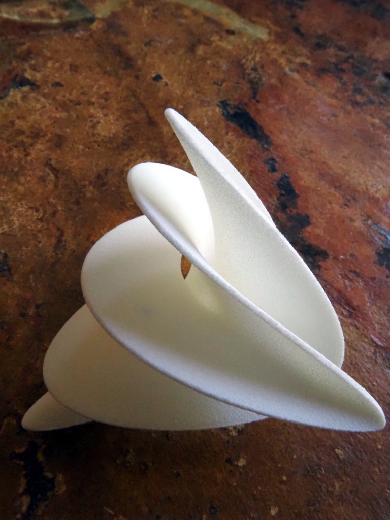
Well, then, let’s select the second, third, and sixth coordinates, assume \(0 \leq r \leq 1\) (the unit disk) and \(0 \leq t \leq 2\pi\) (one full sweep of the parameter plane), and plot or construct the set of points \[ (r^{2}\sin 2t, r^{3}\cos 3t, r^{5}\sin 5t). \] This is the surface whose photograph started the post. The computer plots below show some of the surprising ways this surface appears to change shape as it rotates in space.
In the end, this complicated-looking object has fairly simple complex origins!